
This is a common request: to add some indication of change into something like a bar or column chart. In this case, we’re going to add some little up and down arrows to indicate whether the key value has changed.
So, how do we make this in PowerPoint?
In this how-to, we’ll be using the default sample data PowerPoint gives you, so you can follow along without needing to download anything, but if you want to, you can find the dataset we used to make the example at the top, and a PowerPoint deck with that slide in, and other examples, here:
https://docs.google.com/presentation/d/1JuMc8Inkf8t5snQSVtGp7qffzfGwUbV3?rtpof=true&usp=drive_fs
What you’ll need
Stacked bar
Data manipulation
Chart manipulation
Design tweaks
Custom labeling
How you do it
We’re basically going to create a stacked bar, in which one segment visualizes the data and then use other segments as containers for the custom visuals. We’ll use Excel formulas to create segments for rising and falling values and then use custom fills to add appropriate arrows to those segments.
Details
Add the chart
We’ll start by adding a stacked bar chart. In this case we’ll use the standard stacked bar rather than the 100% option.

PowerPoint will then create an example chart and open Excel to show us the dummy data its populated with.
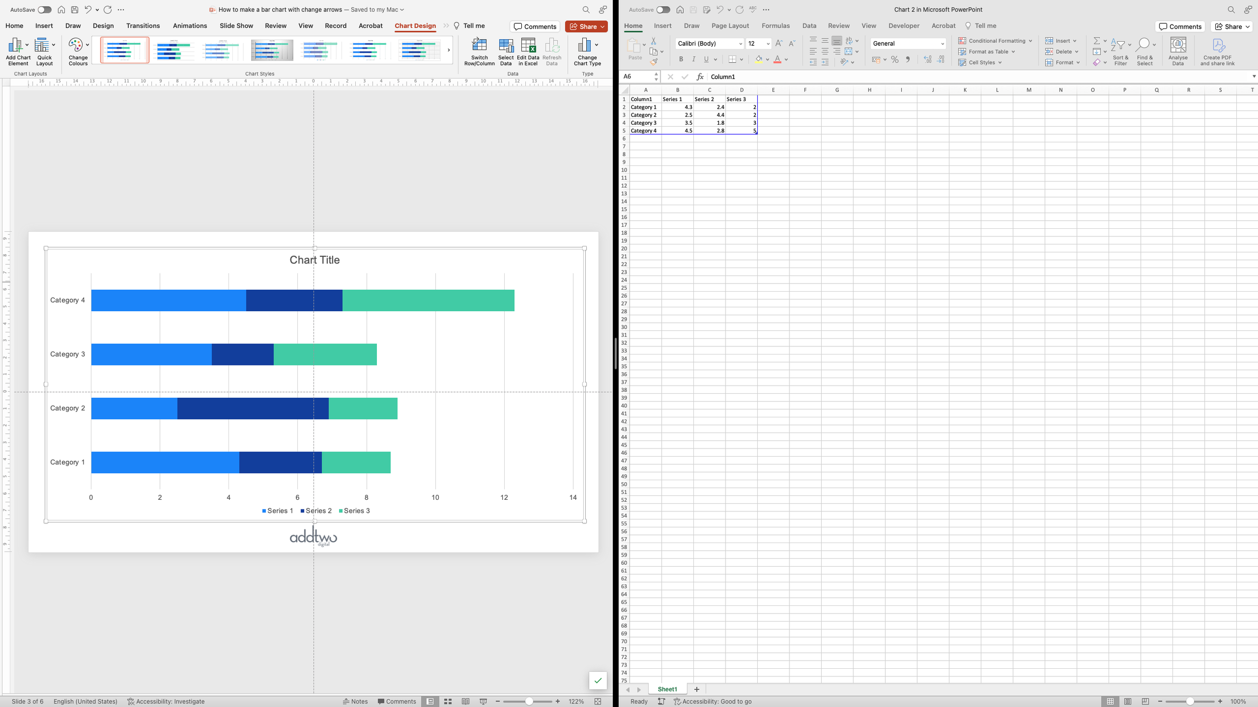
Although PowerPoint opens a whole Excel spreadsheet to show us that data, its only every visualising the section in the blue frame. We can move that around and not affect the chart at all.

However, the spreadsheet still operates as a conventional Excel document. We can add data, formulas and other content to it and it will all be saved in PowerPoint.
Add the data
In this case, we’ll add a table with our actual data in. We’ve got a column of values and then a column of change (from some previous time period, presumably).

Now we’re going to add a formula. What we’re going to want to do is to have one data series that shows our values and then a data series (or two) that contain our arrows. But we want the latter to line up neatly, which means we’re going to want a series in between to make a gap to even everything out.
We’re going to calculate this based on the maximum value in our values series. We can use the Excel MAX() function to do this.

Calculate values to visualise
We’re then going to create rows for all our values inside the blue frame, to add them to our chart. We can name our categories by simply referring to our data table, using the Excel ‘=’ function.

We can do the same to add a column of our actual values.

This then gives us our basic bar chart of our data.

But now we’re going to add a gap at the end of each bar so that our arrows will line up vertically.
We’re going to calculate this by subtracting the value of the data point from the maximum we found earlier, so the formula will look something like:
=SUM($E$2-G2)Don’t forget that adding the ‘$’ to cell references will mean that Excel won’t try and update the reference when you copy it down a column. Instead it will stay referring to a specific cell. The other reference, however, will update to refer to all the cells in our Value column.

This then gives us a set of bars with equal totals: the values and then the remainder of that value subtracted from the maximum.
Add data series for arrows
We’re then going to create a data series for each kind of marker we want to add. We’ll want an arrow for positive change, so we’ll add a data column for that.
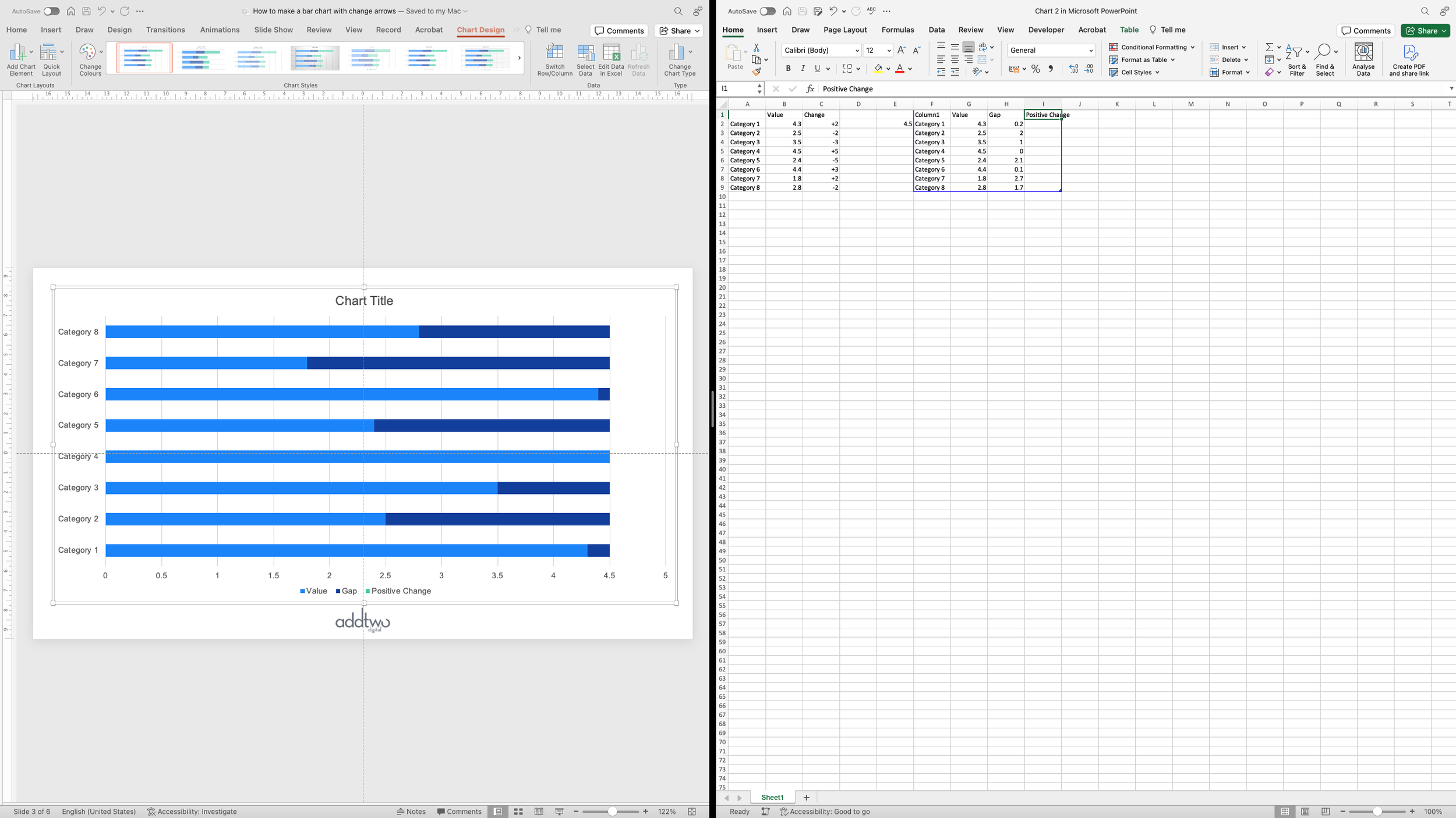
Now we want to fill those cells only if we have a positive change in our change column.
We can do this easily but using an Excel IF() statement. They take the form of IF(thing to test, do this if that’s true, do this if its false). In this case, IF (change is positive, add a value to this cell, otherwise don’t add anything).
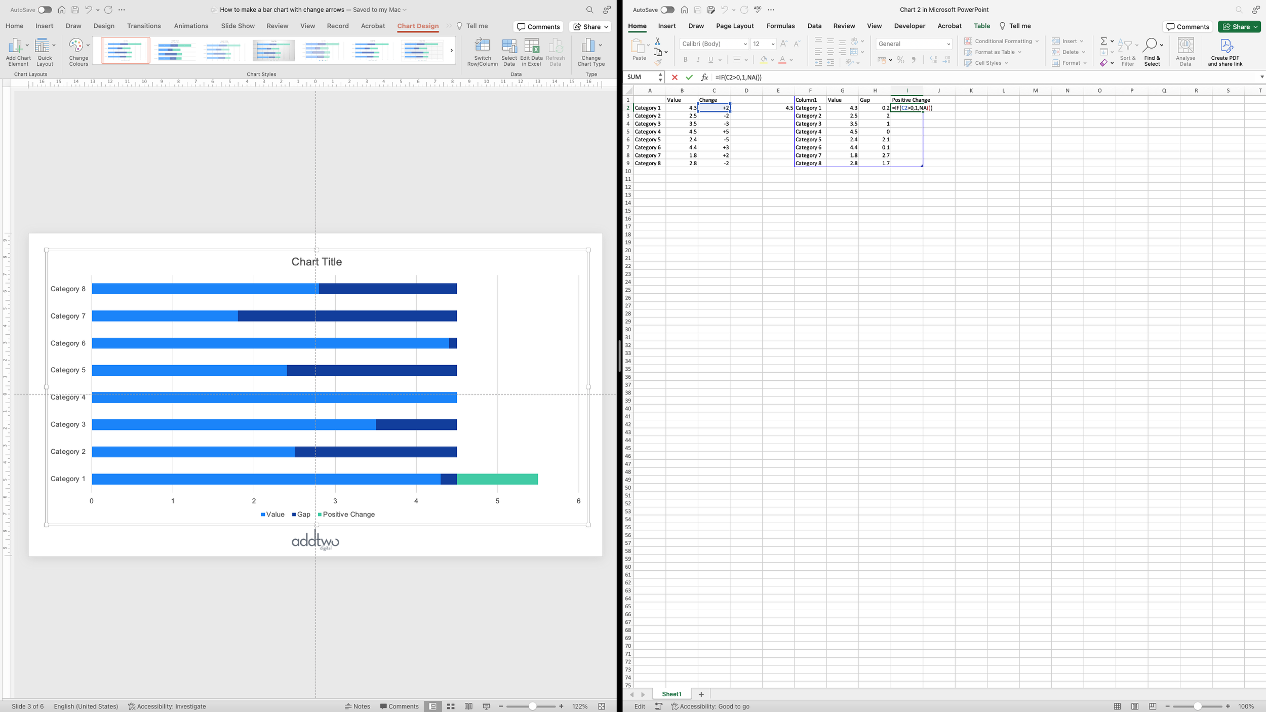
The value we’re going to add if it’s true is totally arbitrary and depends on the rest of the chart. Basically we want a section of bar long enough to contain an arrow and a data label. We can devise a formula to calculate this, but in this case we’ll just set it to ‘1’.
So our resulting IF() statement will look something like this:
=IF(C2>0,1,NA())That NA() simply defines a cell as not having a value in it at all, stopping PowerPoint from visualising anything.
We’re then going to want to do the reverse for negative change - testing to see whether the change is negative and filling those cells with the value ‘1’:
IF(C2<0,1,NA())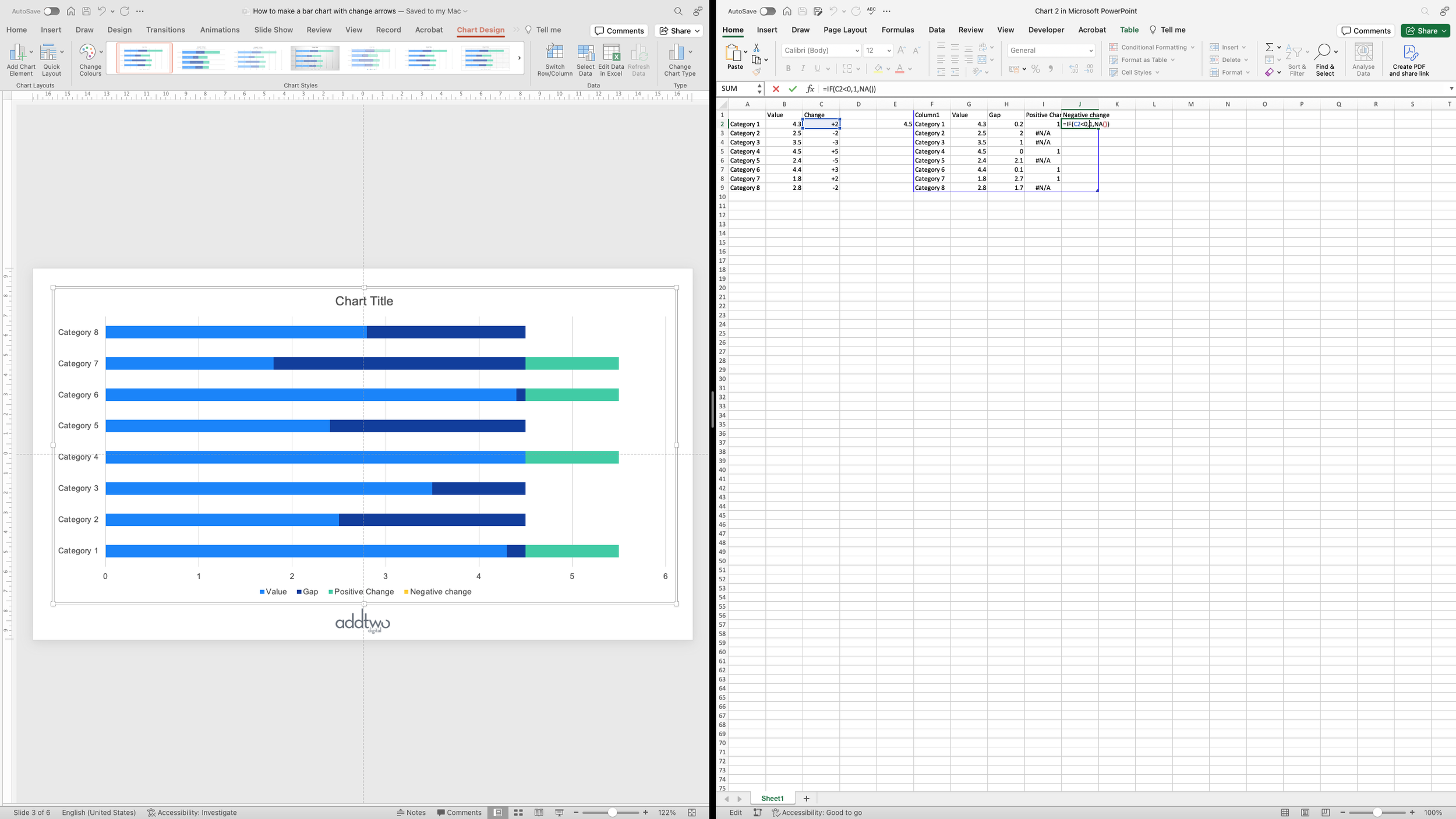
You can see that this then ends each bar with an equally sized section, but in two different data series. PowerPoint has coloured these using default colours from our palette: green and yellow.

We’re also going to add a column for where there’s no change:
=IF(C2=0,1,NA())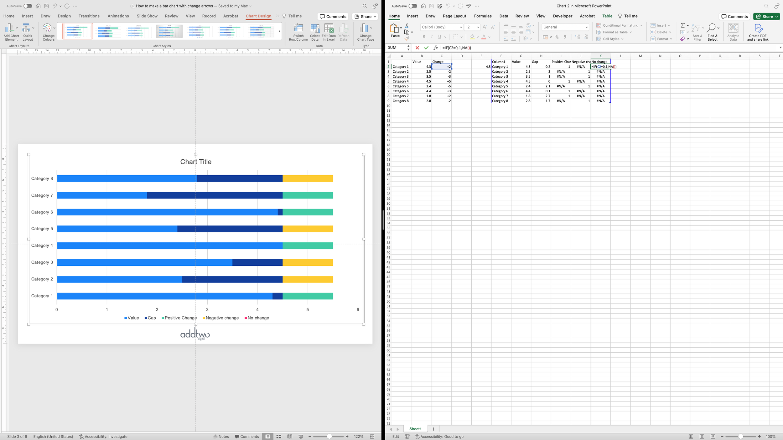
In this case, this makes no difference, as all the values have changed, but it could prove useful in the future.
Now we've done all we need to do with the data - for the moment - and we can close the Excel spreadsheet.
Layout the chart
To start with we need to get the basics of the chart sorted out. We can start by getting the vertical axis in the right order (PowerPoint always reverses the order from the data for some reason).
We can do this in the Format Pane. To open we can right click on the axis and select ‘Format Axis’.
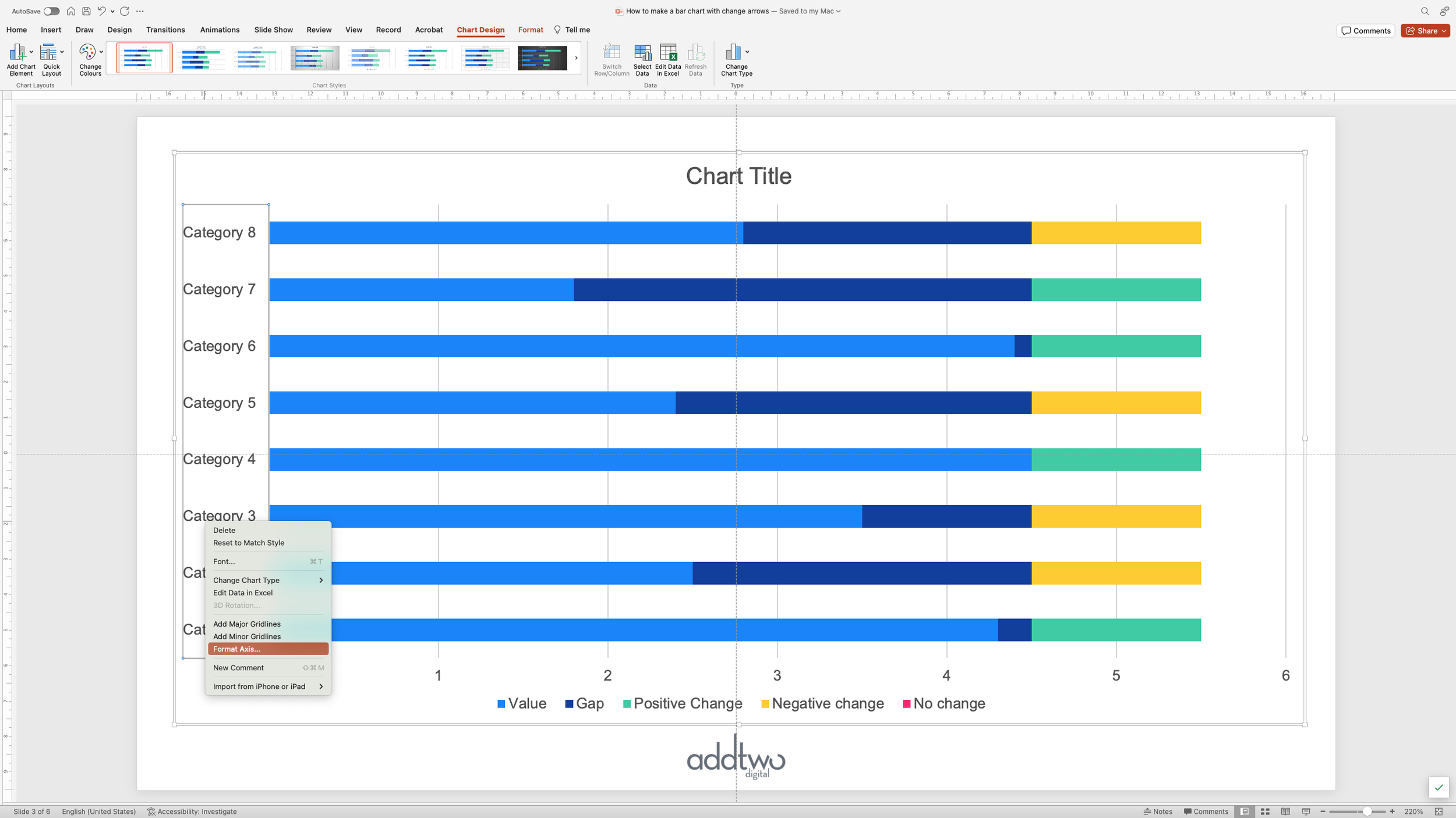
We can then just tick the ‘Categories in reverse order’ to flip the axis the right way up.

While we’ve got that open, let’s remove the axis line from the y-axis, as its entirely superfluous. We can do this by clicking on the Paint Pot icon in the Format Pane and then selecting ‘No line’ under the Line options.

There’s a bunch of other chart elements that we don’t need too.
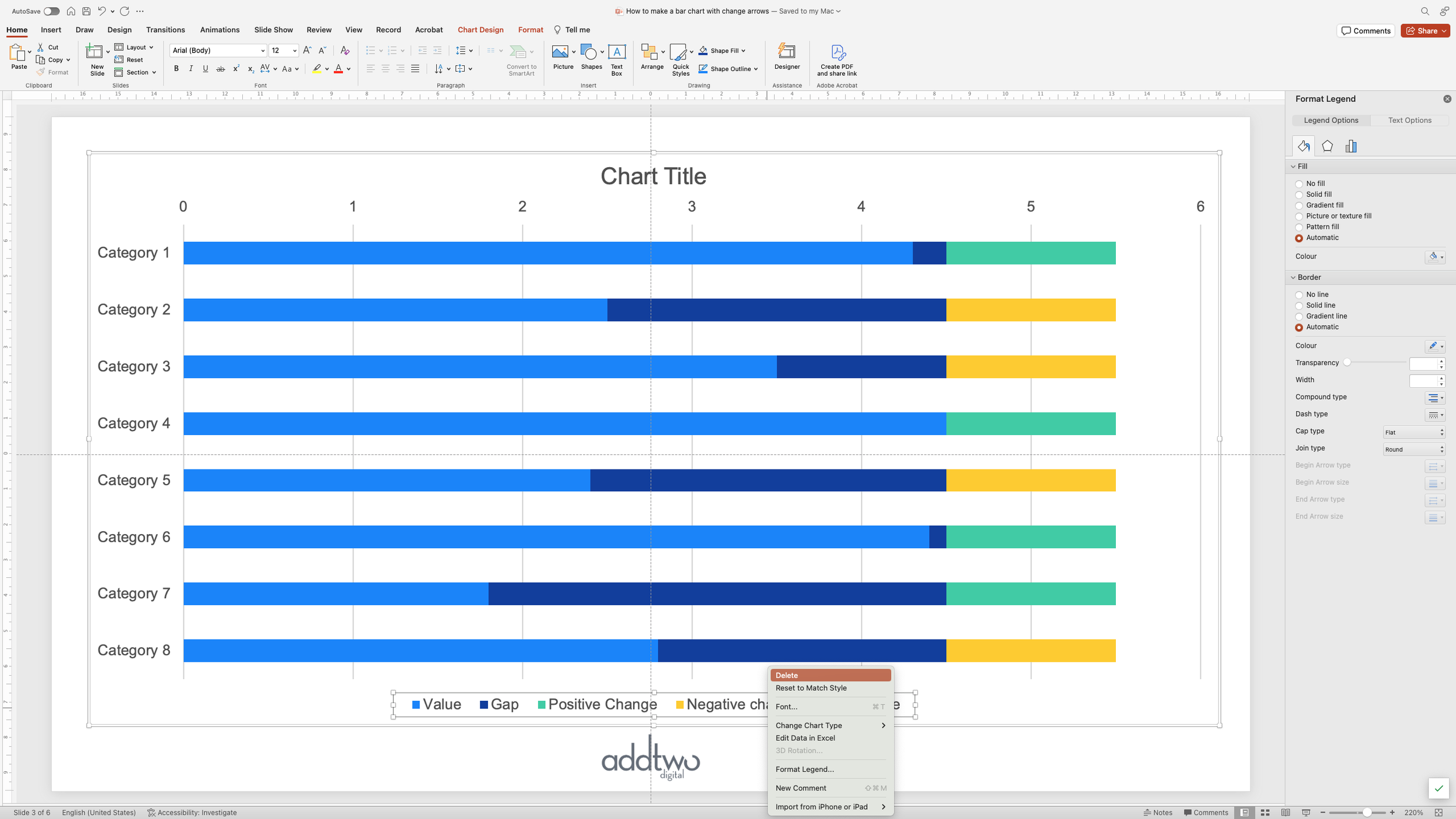
Because we’ve manipulated the data to make the chart, the legend doesn’t help, so we can get rid of that. We can just select it and hit delete, or right-click and select ‘Delete’.
Another way to delete things is to untick them in the ‘Add Chart Element’ menu, which we’ll do to the horizontal axis and the gridlines.

the chart
Now we’ve got the basics out of the way, we can concentrate on the visualisation. To begin with we want to make our ‘gap’ data series at the end of each bar go away.
We can do this by selecting the data series and selecting ‘No Fill’ in the Fill options. You can do this in a number of ways, in the Format Pane, for instance, or just using the usual Fill tools in the ribbon.

Add the arrows
Now we can add the arrows. This means creating a custom fill.
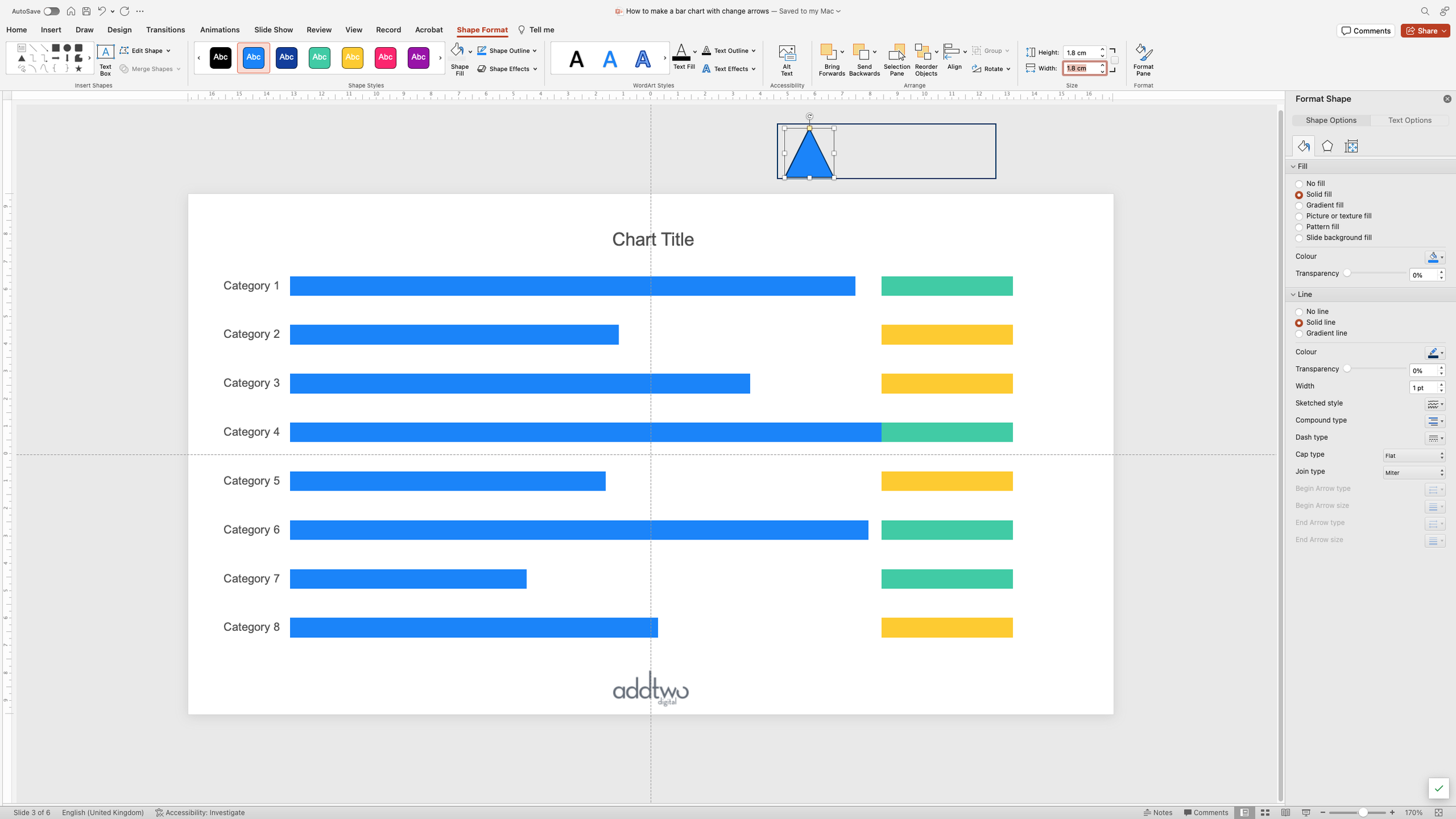
We can start by adding a rectangle using the Shape menu in the Insert tab on the ribbon.

We can set that rectangle to be roughly the same proportions as the blocks for the change data series that we added in the spreadsheet - the green and yellow segments in our chart.

Then we’re going to remove the fill colour from that rectangle by setting it to ‘No Fill’.

Now we’re going to add our arrow for positive change. We’re going to just use an upward pointing triangle.

We’re going to want to position that triangle over the rectangle background we’ve made.
We can then fill that triangle with whatever colour we want to use for positive change.

And we’re going to want to make sure that it’s properly vertically centred against the rectangle, although we’re going to want to keep it over to the left hand side.

With both still selected we’re then going to remove then going to remove the outlines.

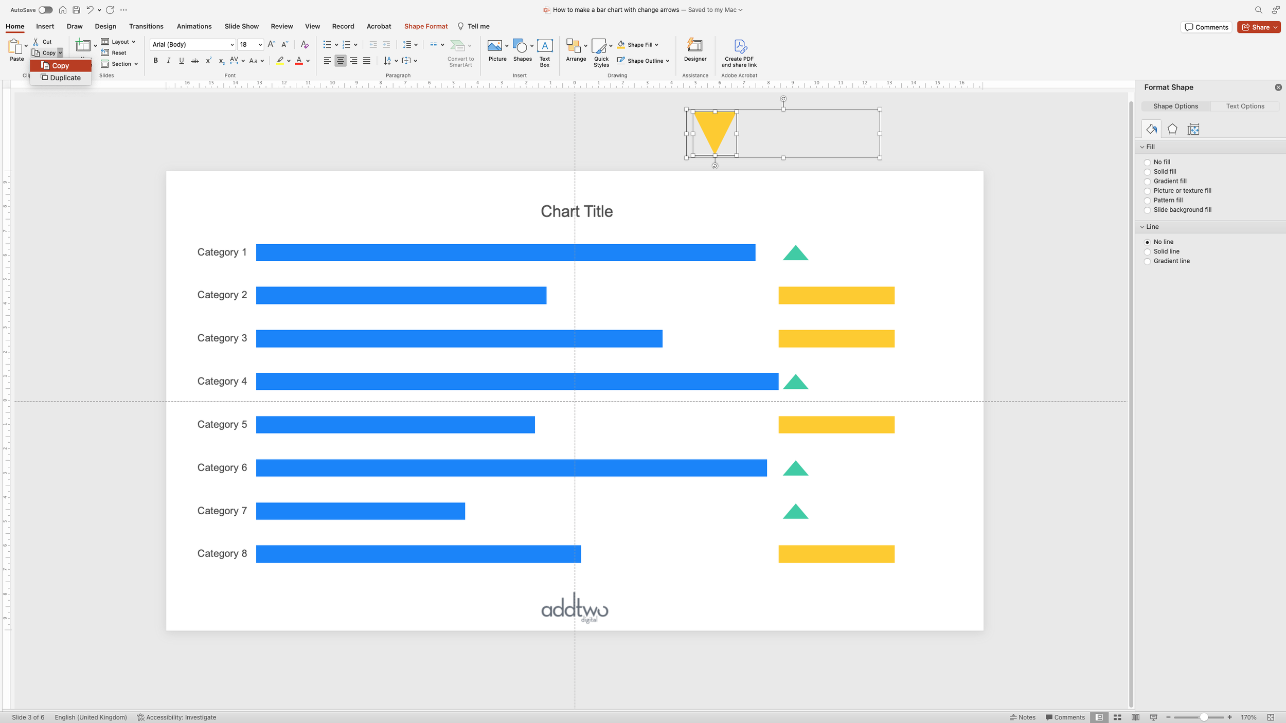
This will leave us with a green triangle against an entirely transparent rectangle. We’re going to want to keep them both selected and copy them both.

Then we want to select the data series for positive change - the green series in our example - and open the Format Pane. We can do this by right-clicking on any data point from that series and selecting ‘Format Data Series’.

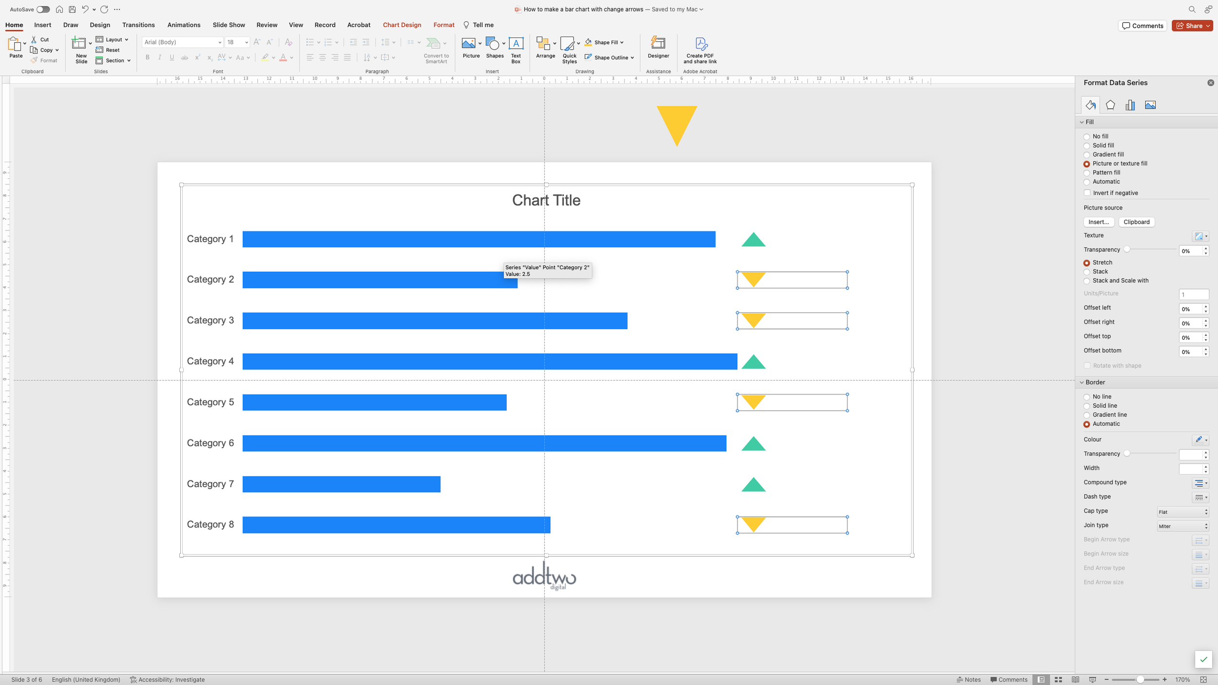
Then, under the Fill options, we’re going to selecting ‘Picture or texture fill’. By default this will fill all this data series with a picture of a canvas texture.

Underneath, however, there are ‘Picture source’ options and we can just click on ‘Clipboard’ to fill the bars with the shapes we just copied.

As you can see, we added the rectangle in the background to give us a bar fill that just features a triangle on the left, with everything else being transparent. Everything’s a bit distorted at the moment, but we’ll get to that.
First we want to add arrows for the negative change. We can do this in exactly the same way. Let’s recolour that triangle for negative change.

And then invert it so it’s pointing downwards.

Then we’re going to select both it and the invisible rectangle (the easiest thing is to just drag around them both) and copy them.
Then we’ll select the negative change data series.

And do the same as the positive change - fill from the clipboard.
And we have our up and down arrows for change.
One more thing, let’s tweak those proportions. Basically, our bars ought to be closer together. We can set this in the Series Options in the Format Pane. By lowering the Gap Width we make the bars wider, which gets the proportions of the triangles looking nicer.

Add labels
We also need some data labels. The labels for the main bars are easy: just right-click on the bars and select ‘Add Data Labels’.

We can then format those labels in the Format Pane by right-clicking on them and selecting ‘Format Data Labels’.

We can set them to appear Inside End on the bars and set the text colour to contrast against the bar fill.

We’re then going to do the same with the change segments. We can right-click on the positive change arrows and select ‘Add Data Labels’.
But these labels are just going to read ‘1’, as that was the default value we gave to all these segments. We can change that though.
We can start by opening the Format Pane for these labels.

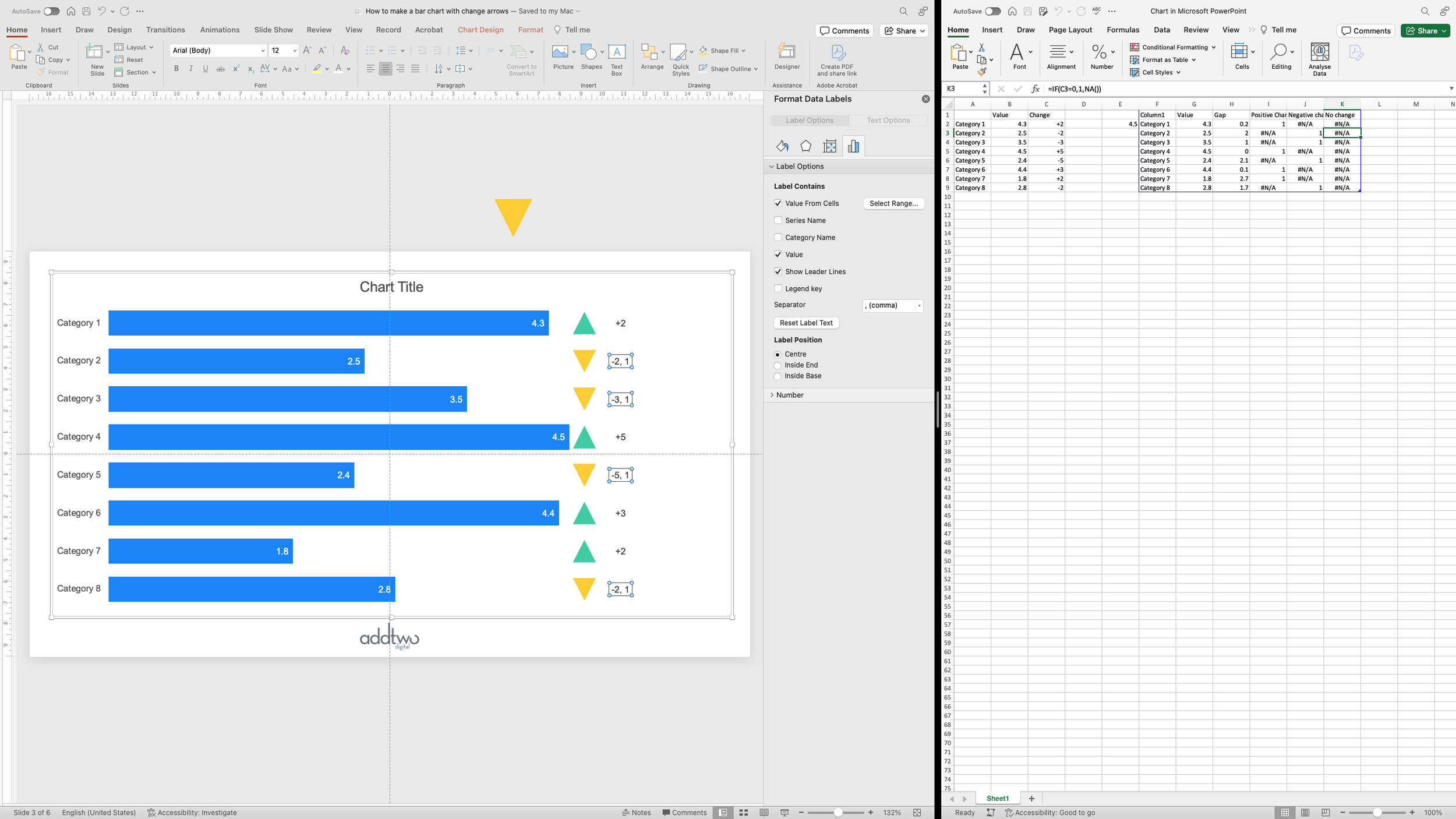
Then, in the Label Contains options, we’re going to select ‘Value From Cells’ options. This will open the Excel spreadsheet with the chart data in. It will then open a dialog box and ask us to select a cell range to use as labels.

We’re going to use our original column of change values.

We can then untick all the other options - these are the only labels we want. Because we’ve set the bars with no positive change to NA(), PowerPoint doesn’t try and label them.

Because we’ve set up the positive and negative changes as separate data series, we’re going to have to repeat this operation for the negative change too.

We’ll select the same column for our Value From Cells labels, and this will then add the negative labels to this data series.
So that’s how we make that in PowerPoint
The hardest part of making these is getting the arrow data series and the arrow graphics themselves the right size, so they look good once they’re added to the chart. It may take some tweaking, especially if you’re making something that you’re going to want to reuse, but it’s worth it.
The great advantage of these change arrows is that they allow you to emphasise the main values but still add in the change. It’s always better to add a separate visualisation rather than just keep trying to shoehorn in elements onto a chart until the whole thing becomes impossible to understand.
